Matplotlib基础

Matplotlib是一个用于Python编程语言的绘图库,它提供了一个面向对象的API,可以生成多种静态、交互式和动画可视化。Matplotlib可以用来创建高质量的图表,如线图、散点图、条形图、饼图、柱状图、误差线图、箱线图、3D 图表等等。
第一章 课程绪论
1.1 数据分析及可视化概念
数据分析是指用适当的统计分析方法对收集来的大量数据进行分析,提取有用信息和形成结论而对数据加以详细研究和概括总结的过程
收集数据 - 提取信息 - 形成结论
借助图形化手段表示数据,即为数据可视化的过程。
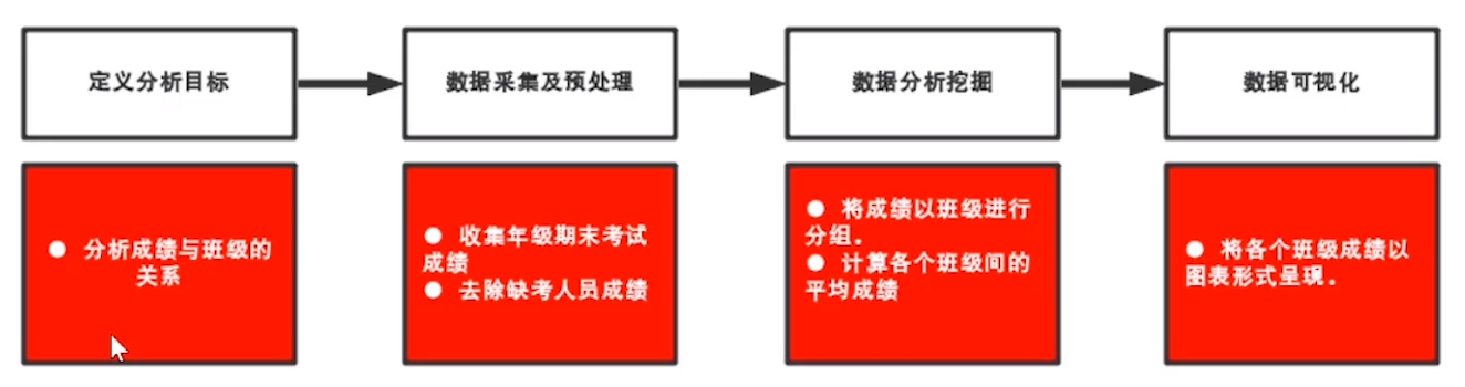
1.2 数据分析可视化流程
(1).定义分析目标
(2).数据采集及预处理
(3).数据分析挖掘
(4).数据可视化
数据清洗:数据清洗是指发现并纠正数据文件中可识别的错误的最后一道程序,包括检查数据一致性,处理无效值和缺失值等。
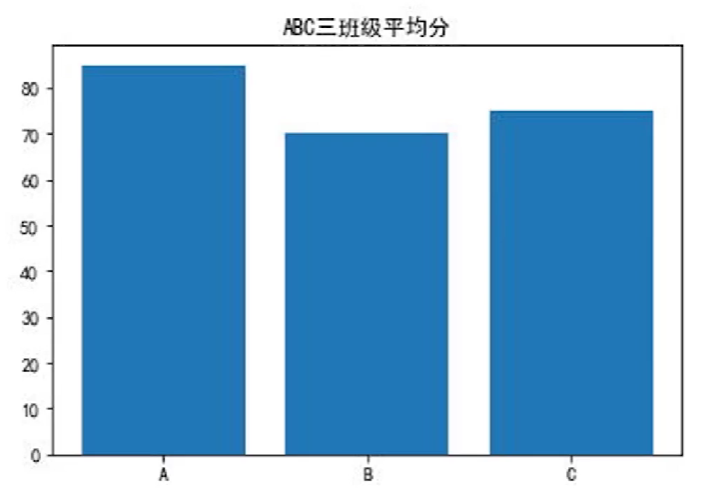
1.3 数据分析可视化案例
数据分析常用于商业决策,挖掘消费模式,优化资源配置以达到利益最大化。为了使数据更加直观清晰的呈现在人们面前,我们需要考虑用合适的方式和方法对数据进行可视化处理
(1)电影院以电影放映时间和入座率的时间序列模型进行排片
(2)网店挖掘商品售卖记录进行更科学的定价
(3)城市根据交通情况绘制热力图,优化出行效率。


1.4 常见的可视化形式及工具
1.4.1 可视化形式:
统计图 (直方图,折线图,饼图)
分布图 (热力图,散点图,气泡图)
1.4.2 常用工具
| 分类 | 软件名称 |
|---|---|
| 分析工具 | pandas,SciPy,numpy,sklearn |
| 绘图工具 | matplotlib, Pychart, reportlab |
| 平台工具 | Jupyter Notebook,PyCharm |
Matplotlib 是 Python 的绘图库。它可与 NumPy 一起使用提供了一种有效的 MatLab 开源替代方案。 它也可以和图形工具包一起使用,如 PyQt和 wxPython。
![]()
Jupyter Notebook是一个交互式笔记本,支持运行 40 多种编程语言。其本质是一个 Web 应用程序,便于创建和共享文学化程序文档,支持实时代码,数学方程,可视化和 markdown用途包括:数据清理和转换,数值模拟,统计建模,机器学习等等。
第二章 环境安装
2.1 安装Anaconda
Anaconda是专业的数据科学计算环境,已经集成绝大部分包和工具,可以用于在同一个机器上安装不同版本的软件包及其依赖,并能够在不同的环境之间切换,不需要多余调试,使用方便。
Anaconda官网:https://www.anaconda.com/
2.2 配置使用Jupyter Notebook
Jupyter Notebook是基于网页的用于交互计算的应用程序。其可被应用于全过程计算:开发、文档编写、运行代码和展示结果。
- conda创建新的python环境并启用
- conda安装Jupyter Notebook
- 启动Jupyter Notebook
2.2.1 配置
在Anaconda Prompt输入如下命令:
1 | conda create -n myPython python=3.7 |
2.3 安装matplotlib
Matplotlib 是一个 Python 的 2D绘图库,它以各种硬拷贝格式和跨平台的交互式环境生成出版质量级别的图形。
- 启用conda环境
- 安装matplotlib
1 | pip install matplotlib |
- 绘制第一个图形
1 | import matplotlib |
第三章 matplotlib入门
3.1 matplotlib配置讲解
3.1.1 matplotlib.rcParams
rcParams是matplotlib存放设置的字典,修改字典键值以改变matplotlib绘图的相关设置。
https://matplotlib.org/api/matplotlib_configuration_api.html
若不进行基本配置,可能会出现各种小问题,例如无法正常显示中文等。
matplotlib.rcParams常用基本配置
1 | plt.rcParams['font.sans-serif'] = ['SimHei'] # 中文支持 |
1 | import matplotlib |
3.2 绘制直方图,条形图,折线图和饼图
直方图又称质量分布图,是一种统计报告图,由一系列高度不等的纵向条纹或线段表示数据分布的情况。
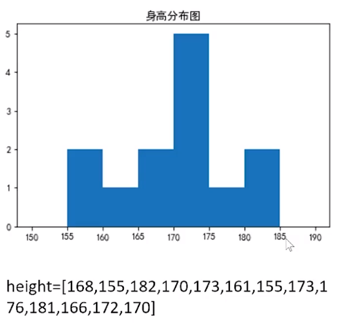
3.2.1 绘制直方图:plt.hist(data)
1 | import matplotlib as mpl |
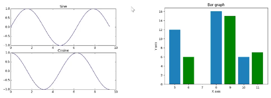
3.2.2 绘制条形图:plt.bar(X,Y)
条形图是用宽度相同的条形的高度或长短来表示数据多少的图形。
1 | import matplotlib.pyplot as plt |
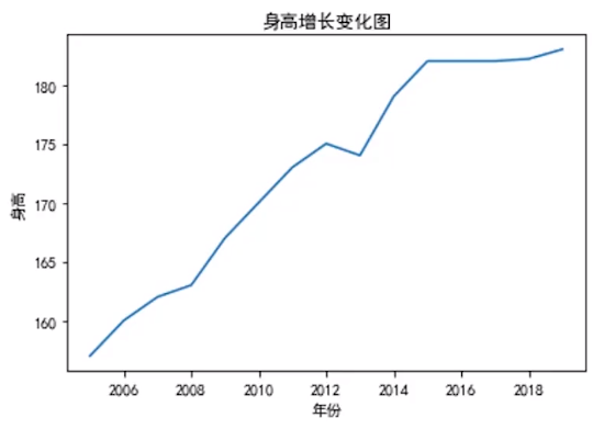
3.2.3 绘制折线图:plt.plot(X,Y)
折线图通常显示随时间而变化的连续数据,因此非常适用于体现在相等时间间隔下数据的趋势。
1 | import matplotlib.pyplot as plt |
3.2.4 绘制饼图:plt.pie(data)
饼图常用于显示一个数据系列中各项的大小与各项总和的比例。
1 | import matplotlib.pyplot as plt |
3.3 绘制散点图和箱线图
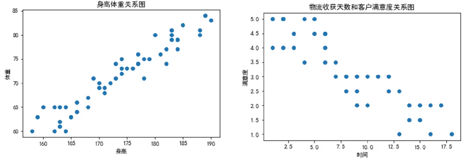
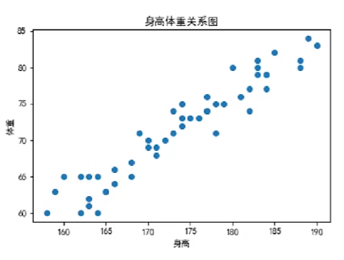
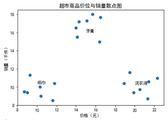
3.3.1 绘制散点图:plt.scatter(x,Y)
散点图是指在回归分析中数据点在直角坐标系平面上的分布图,散点图表示因变量随自变量而变化的大致趋势,据此可以选择合适的函数对数据点进行拟合。
1 | import matplotlib.pyplot as plt |
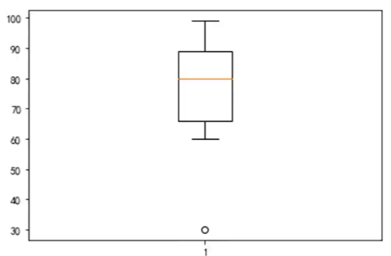
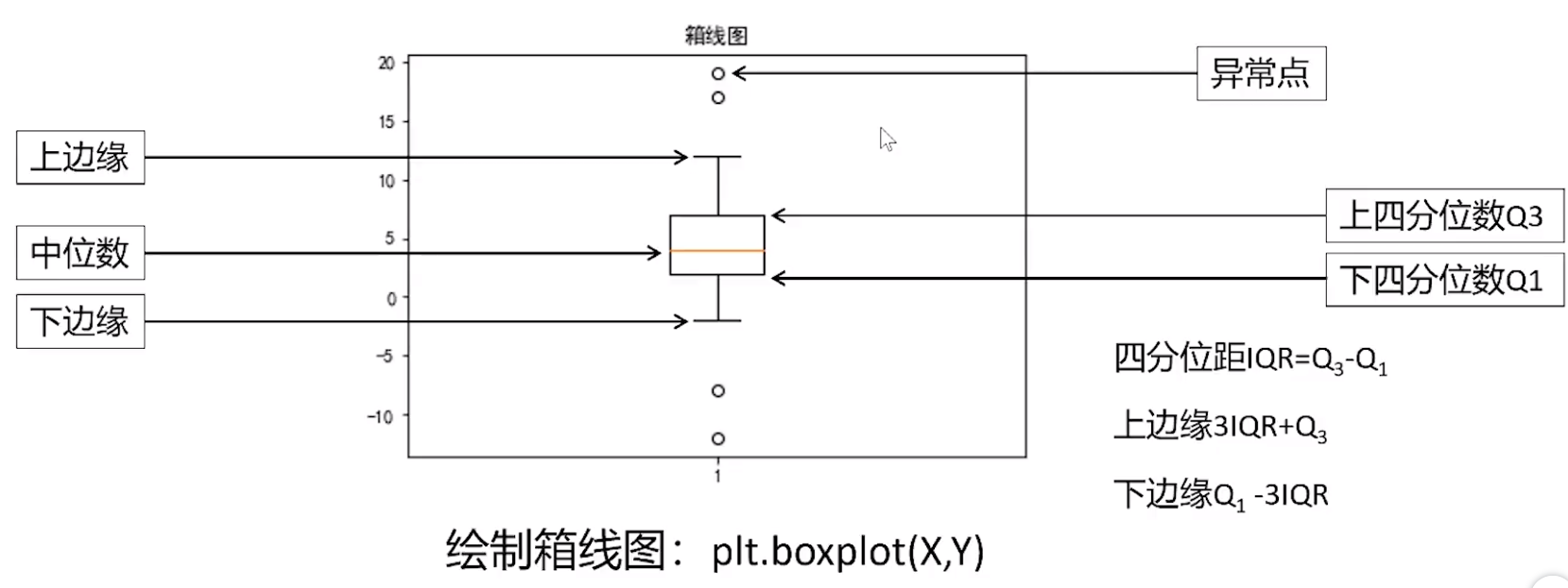
3.3.2 绘制箱线图:plt.boxplot(X,Y)
箱线图又称为盒须图、盒式图,是一种用作显示一组数据分散情况的统计图。主要用于反映原始数据分布的特征。
1 | import matplotlib.pyplot as plt |
3.4 绘制极线图和阶梯图
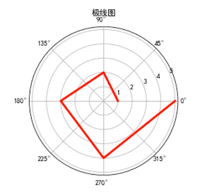
3.4.1 绘制极线图:projection=’polar’
极线图用于表示极坐标下的数据分布情况,多用于显示具有一定周期性的数据。
1 | import matplotlib.pyplot as plt |
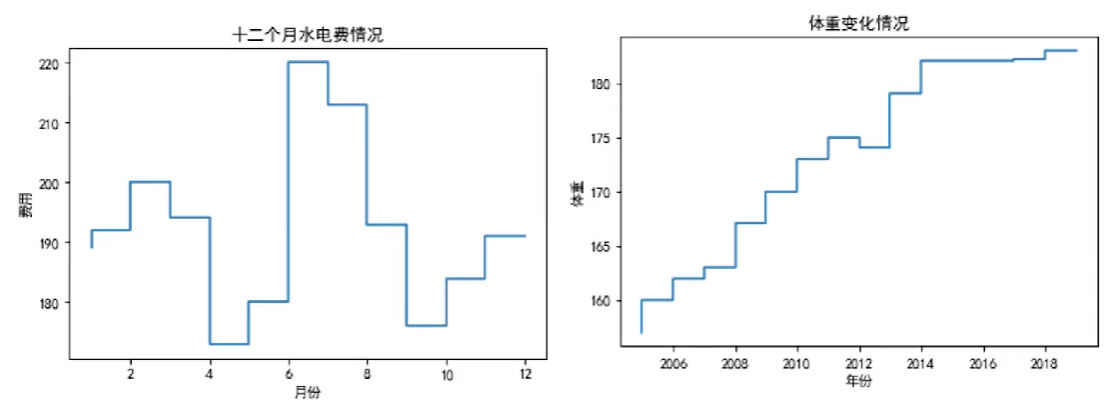
3.4.2 绘制阶梯图\箱线图:plt.step(X, Y)
阶梯图是一种以无规律、间歇型阶跃的方式表达数值变化的方法。它不仅可以像折线图一样反映数据发展的趋势,还可以反映数据状态的持续时间。
1 | import matplotlib.pyplot as plt |
第四章 matplotlib高级图形绘制
4.1 matplotlib图表参数设置
1 | import matplotlib.pyplot as plt |
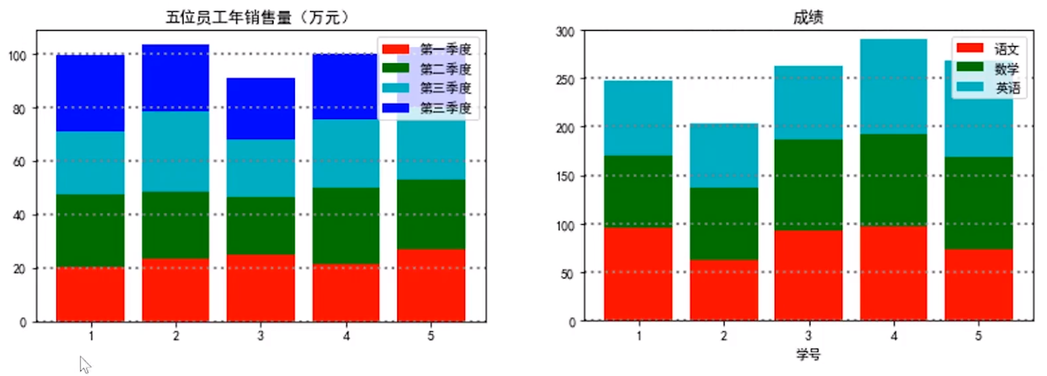
4.2 绘制堆积图
堆积图常用于综合展示不同分类的指标趋势以及它们的总和的趋势。比如说,我们想看一下5名同学期末的总分情况,同时我们又想看一下这5名同学的各科成绩以及它们各自的占比,这时,我们就可以用堆积图来更高效、更简洁地展示出来,
1 | import matplotlib.pyplot as plt |
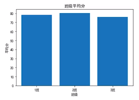
4.3 绘制分块图
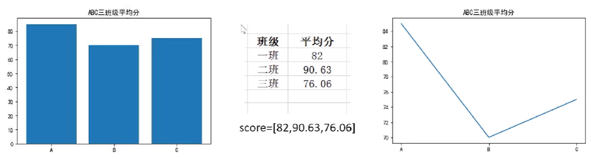
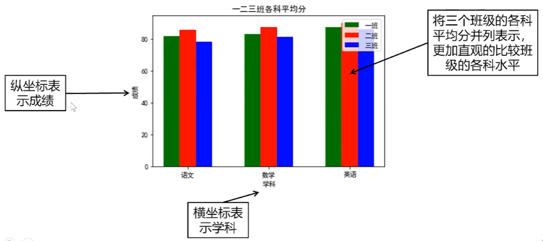
分块图可将不同数据集进行并列显示,通常可用于对同一方面的不同主体进行比较(例如用分块图来比较1班,2班,3班的各科平均分情况)
1 | import matplotlib.pyplot as plt |
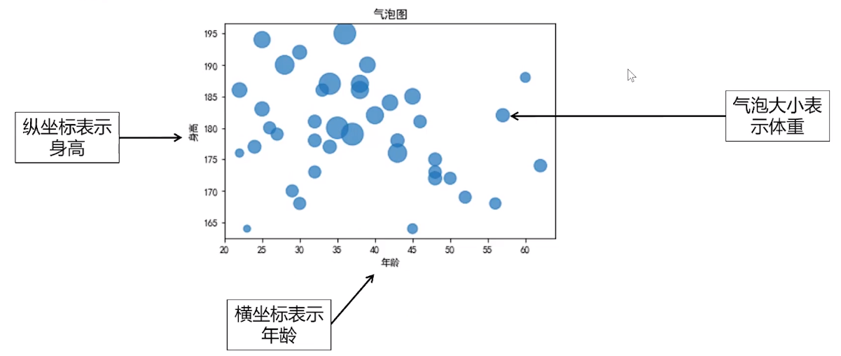
4.4 绘制气泡图
1 | import matplotlib.pyplot as plt |
第五章 matplotlib综合系例
5.1 项目介绍
显示各省份的降雪情况
5.2 数据处理分析
1 | import matplotlib.pyplot as plt |
5.3 可视化输出结果
1 | import matplotlib.pyplot as plt |